Implementing an equation of state in python
In FeOs, you can implement your equation of state in python, register it to the Rust backend, and compute properties and phase equilbria as if you implemented it in Rust. In this tutorial, we will implement the Peng-Robinson equation of state.
Table of contents
Phase equilibria and phase diagrams
Comparison to Rust implementation
[1]: importfeosimportsi_unitsassiimportnumpyasnpoptional=Trueimportwarningswarnings.filterwarnings('ignore')ifoptional:importmatplotlib.pyplotaspltimportpandasaspdimportseabornassnssns.set_style("ticks")sns.set_palette("Dark2")sns.set_context("talk")Implementation
To implement an equation of state in python, we have to define a class which has to have the following methods:
classMyEquationOfState:defhelmholtz_energy(self,state:StateHD)->Ddefcomponents(self)->intdefsubset(self,indices:List[int])->Selfdefmolar_weight(self)->SIArray1defmax_density(self,molefracs:np.ndarray[float])->floatcomponents(self)->int: Returns the number of components (usually inferred from the shape of the input parameters).
molar_weight(self)->SIArray1: Returns an SIArray1 with size equal to the number of components containing the molar mass of each component.
max_density(self,moles:np.ndarray[float])->float: Returns the maximum allowed number density in units of molecules/Angstrom³.
subset(self,indices:List[int])->self: Returns a new equation of state with parameters defined in indices.
helmholtz_energy(self,state:StateHD)->Dual: Returns the helmholtz energy as (hyper)-dual number given a StateHD.
[2]: SQRT2=np.sqrt(2)classPyPengRobinson:def__init__(self,critical_temperature,critical_pressure,acentric_factor,molar_weight,delta_ij=None):"""Peng-Robinson Equation of State Parameters ---------- critical_temperature : SIArray1 critical temperature of each component. critical_pressure : SIArray1 critical pressure of each component. acentric_factor : np.array[float] acentric factor of each component (dimensionless). molar_weight: SIArray1 molar weight of each component. delta_ij : np.array[[float]], optional binary parameters. Shape=[n, n], n = number of components. defaults to zero for all binary interactions. Raises ------ ValueError: if the input values have incompatible sizes. """self.n=len(critical_temperature)iflen(set((len(critical_temperature),len(critical_pressure),len(acentric_factor))))!=1:raiseValueError("Input parameters must all have the same lenght.")self.tc=critical_temperature/si.KELVINself.pc=critical_pressure/si.PASCALself.omega=acentric_factorself.mw=molar_weight/si.GRAM*si.MOLself.a_r=(0.45724*critical_temperature**2*si.RGAS/critical_pressure/si.ANGSTROM**3/si.NAV/si.KELVIN)self.b=(0.07780*critical_temperature*si.RGAS/critical_pressure/si.ANGSTROM**3/si.NAV)self.kappa=(0.37464+(1.54226-0.26992*acentric_factor)*acentric_factor)self.delta_ij=(np.zeros((self.n,self.n))ifdelta_ijisNoneelsedelta_ij)defhelmholtz_energy(self,state):"""Return helmholtz energy. Parameters ---------- state : StateHD The thermodynamic state. Returns ------- helmholtz_energy: float | any dual number The return type depends on the input types. """x=state.molefracstr=1.0/self.tc*state.temperatureak=((1.0-np.sqrt(tr))*self.kappa+1.0)**2*self.a_rak_mix=0.0ifself.n>1:foriinrange(self.n):forjinrange(self.n):ak_mix+=(np.sqrt(ak[i]*ak[j])*(x[i]*x[j]*(1.0-self.delta_ij[i,j])))else:ak_mix=ak[0]b=np.sum(x*self.b)rho=np.sum(state.partial_density)a=rho*(-np.log(1.0-b*rho)-ak_mix/(b*SQRT2*2.0*state.temperature)*np.log((1.0+(1.0+SQRT2)*b*rho)/(1.0+(1.0-SQRT2)*b*rho)))returnadefcomponents(self)->int:"""Number of components."""returnself.ndefsubset(self,i:list[int]):"""Return new equation of state containing a subset of all components."""ifself.n>1:tc=self.tc[i]pc=self.pc[i]mw=self.mw[i]omega=self.omega[i]returnPyPengRobinson(si.array(tc*si.KELVIN),si.array(pc*si.PASCAL),omega,si.array(mw*si.GRAM/si.MOL))else:returnselfdefmolar_weight(self)->si.SIObject:returnsi.array(self.mw*si.GRAM/si.MOL)defmax_density(self,molefracs:list[float])->float:b=np.sum(molefracs*self.b)return0.9/bComputing properties
Let’s compute some properties. First, we have to instanciate the class and register it to Rust. This is done using the EquationOfState.python method.
[3]: tc=si.array(369.96*si.KELVIN)pc=si.array(4250000.0*si.PASCAL)omega=np.array([0.153])molar_weight=si.array(44.0962*si.GRAM/si.MOL)# create an instance of our python class and hand it over to rustpr=PyPengRobinson(tc,pc,omega,molar_weight)eos=feos.EquationOfState.python_residual(pr)Thermodynamic state: the State object
Before we can compute a property, we create a State object. This can be done in several ways depending on what variables are specified. If no total amount of substance is defined, the state can only be used to calculate intesive properties. For possible input combinations, you can inspect the signature of the constructor using State?.
[4]: feos.State?Init signature: feos.State( eos, temperature=None, volume=None, density=None, composition=None, pressure=None, molar_enthalpy=None, molar_entropy=None, molar_internal_energy=None, density_initialization=None, initial_temperature=None, ) Docstring: A thermodynamic state at given conditions. Parameters ---------- eos : Eos The equation of state to use. temperature : SINumber, optional Temperature. volume : SINumber, optional Volume. density : SINumber, optional Molar density. composition : float | SINumber | numpy.ndarray[float] | SIArray1 | list[float], optional Composition of the mixture. pressure : SINumber, optional Pressure. molar_enthalpy : SINumber, optional Molar enthalpy. molar_entropy : SINumber, optional Molar entropy. molar_internal_energy: SINumber, optional Molar internal energy density_initialization : {'vapor', 'liquid', SINumber, None}, optional Method used to initialize density for density iteration. 'vapor' and 'liquid' are inferred from the maximum density of the equation of state. If no density or keyword is provided, the vapor and liquid phase is tested and, if different, the result with the lower free energy is returned. initial_temperature : SINumber, optional Initial temperature for temperature iteration. Can improve convergence when the state is specified with pressure and molar entropy or enthalpy. Returns ------- State : state at given conditions Raises ------ Error When the state cannot be created using the combination of input. Type: type Subclasses:If we use input variables other than \(\mathbf{N}, V, T\) (the natural variables of the Helmholtz energy), creating a state is an iterative procedure. For example, we can create a state for a give \(T, p\), which will result in a iteration of the volume (density).
[5]: s=feos.State(eos,temperature=300*si.KELVIN,pressure=1*si.BAR)s.density[5]: $40.755\,\mathrm{\frac{ mol}{m^{3}}}$
[6]: # The `composition` argument is used to specify the composition AND total amount based on the unit of the argument.# With the total amount specified, extensive properties can be evaluated.s_pt=feos.State(eos,temperature=300*si.KELVIN,pressure=1*si.BAR,composition=1*si.MOL)s_pt.total_moles,s_pt.helmholtz_energy(feos.Contributions.Residual)[6]: (1 mol, -40.78921616151256 J) Critical point
To generate a state at critical conditions, we can use the critical_point constructor.
[7]: s_cp=feos.State.critical_point(eos)print("Critical point")print("temperature: ",s_cp.temperature)print("density : ",s_cp.mass_density())print("pressure : ",s_cp.pressure())Critical point temperature: 369.9506174234607 K density : 198.1862458057178 kg/m³ pressure : 4.249677749116937 MPa Phase equilibria and phase diagrams
We can also create an object, PhaseEquilibrium, that contains states that are in equilibrium.
[8]: vle=feos.PhaseEquilibrium.pure(eos,300.0*si.KELVIN)vle[8]: temperature
density
phase 1
300.00000 K
488.99014 mol/m³
phase 2
300.00000 K
11.53399 kmol/m³
Each phase is a State object. We can simply access these states and compute properties, just like before.
[9]: vle.liquid# the high density phase `State`[9]: temperature
density
300.00000 K
11.53399 kmol/m³
[10]: vle.vapor# the low density phase `State`[10]: temperature
density
300.00000 K
488.99014 mol/m³
[11]: # we can now easily compute any property:print("Heat of vaporization: ",vle.vapor.molar_enthalpy(feos.Contributions.Residual)-vle.liquid.molar_enthalpy(feos.Contributions.Residual))print("for T = {}".format(vle.liquid.temperature))print("and p = {:.2f} bar".format(vle.liquid.pressure()/si.BAR))Heat of vaporization: 14.782343503305128 kJ/mol for T = 300 K and p = 9.95 bar We can also easily compute vapor pressures and boiling temperatures:
[12]: # This also works for mixtures, in which case the pure component properties are computed.# Hence, the result is a list - that is why we use an index [0] here.print("vapor pressure (T = 300 K):",feos.PhaseEquilibrium.vapor_pressure(eos,300*si.KELVIN)[0])print("boiling temperature (p = 3 bar):",feos.PhaseEquilibrium.boiling_temperature(eos,2*si.BAR)[0])vapor pressure (T = 300 K): 994.7761635610082 kPa boiling temperature (p = 3 bar): 247.84035574956755 K Phase Diagram
We could repeatedly compute PhaseEquilibrium states for different temperatures / pressures to generate a phase diagram. Because this a common task, there is a object for that as well.
The PhaseDiagram object creates multiple PhaseEquilibrium objects (npoints of those) between a given lower temperature and the critical point.
[13]: dia=feos.PhaseDiagram.pure(eos,230.0*si.KELVIN,500)We can access each PhaseEquilbrium and then conveniently comput any property we like:
[14]: enthalpy_of_vaporization=[(vle.vapor.molar_enthalpy(feos.Contributions.Residual)-vle.liquid.molar_enthalpy(feos.Contributions.Residual))/(si.KILO*si.JOULE)*si.MOLforvleindia.states][15]: fig,ax=plt.subplots(figsize=(7,4))sns.lineplot(x=dia.vapor.temperature/si.KELVIN,y=enthalpy_of_vaporization,ax=ax);ax.set_ylabel(r"$\Delta^{LV}h$ / kJ / mol")ax.set_xlabel(r"$T$ / K");

A more convenient way is to create a dictionary. The dictionary can be used to build pandas DataFrame objects. This is a bit less flexible, because the units of the properties are rigid. You can inspect the method signature to check what units are used.
[16]: dia.to_dict?Signature: dia.to_dict(contributions) Docstring: Returns the phase diagram as dictionary. Parameters ---------- contributions : Contributions, optional The contributions to consider when calculating properties. Defaults to Contributions.Total. Returns ------- Dict[str, List[float]] Keys: property names. Values: property for each state. Notes ----- - temperature : K - pressure : Pa - densities : mol / m³ - mass densities : kg / m³ - molar enthalpies : kJ / mol - molar entropies : kJ / mol / K - specific enthalpies : kJ / kg - specific entropies : kJ / kg / K - xi: liquid molefraction of component i - yi: vapor molefraction of component i - component index `i` matches to order of components in parameters. Type: builtin_function_or_method [17]: data_dia=pd.DataFrame(dia.to_dict(feos.Contributions.Residual))data_dia.head()[17]: temperaturepressuredensity liquiddensity vapormolar enthalpy liquidmolar enthalpy vapormolar entropy liquidmolar entropy vapormass density liquidmass density vaporspecific enthalpy liquidspecific enthalpy vaporspecific entropy liquidspecific entropy vapor0230.00000096625.27817414125.98894752.208491-18.921555-0.157448-0.035166-0.000148622.9024342.302196-429.097170-3.570554-0.797483-0.0033631230.28046297830.13395614118.00685252.811929-18.911909-0.159193-0.035119-0.000150622.5504542.328805-428.878435-3.610123-0.796418-0.0033992230.56092499046.72940014110.01022053.420767-18.902255-0.160952-0.035072-0.000152622.1978332.355653-428.659501-3.650021-0.795354-0.0034363230.841386100275.14312014101.99901154.035036-18.892592-0.162726-0.035025-0.000153621.8445692.382740-428.440366-3.690251-0.794290-0.0034734231.121849101515.45396414093.97318254.654773-18.882920-0.164515-0.034978-0.000155621.4906602.410068-428.221030-3.730814-0.793228-0.003510Once we have a dataframe, we can store our results or create a nicely looking plot:
[18]: defphase_plot(data,x,y):fig,ax=plt.subplots(figsize=(12,6))ifx!="pressure"andx!="temperature":xl=f"{x} liquid"xv=f"{x} vapor"else:xl=xxv=xify!="pressure"andy!="temperature":yl=f"{y} liquid"yv=f"{y} vapor"else:yv=yyl=ysns.lineplot(data=data,x=xv,y=yv,ax=ax,label="vapor")sns.lineplot(data=data,x=xl,y=yl,ax=ax,label="liquid")ax.set_xlabel(x)ax.set_ylabel(y)ax.legend(frameon=False)sns.despine();[19]: phase_plot(data_dia,"density","temperature")
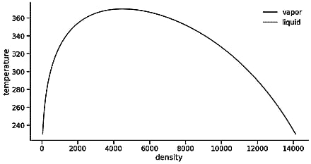
[20]: phase_plot(data_dia,"molar entropy","temperature")
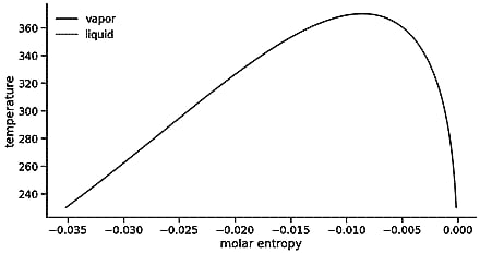
Mixtures
Fox mixtures, we have to add information about the composition, either as molar fraction, amount of substance per component, or as partial densities.
[21]: # propane, butane mixturetc=np.array([369.96,425.2])*si.KELVINpc=np.array([4250000.0,3800000.0])*si.PASCALomega=np.array([0.153,0.199])molar_weight=np.array([44.0962,58.123])*si.GRAM/si.MOLpr=PyPengRobinson(tc,pc,omega,molar_weight)eos=feos.EquationOfState.python_residual(pr)[22]: s=feos.State(eos,temperature=300*si.KELVIN,pressure=1*si.BAR,composition=np.array([0.5,0.5]),)s[22]: temperature
density
molefracs
300.00000 K
40.96869 mol/m³
[0.50000, 0.50000]
As before, we can compute properties by calling methods on the State object. Some return vectors or matrices - for example the chemical potential and its derivative w.r.t amount of substance:
[23]: s.chemical_potential(feos.Contributions.Residual)[23]: array([ -93.60749754, -120.5269973 ]) J/mol [24]: s.n_dmu_dni()/(si.KILO*si.JOULE/si.MOL)[24]: array([[ 4.90721995, -0.10487987], [-0.10487987, 4.85361765]]) Phase equilibria can be built from different constructors. E.g. at critical conditions given composition:
[25]: s_cp=feos.State.critical_point(eos,composition=np.array([0.5,0.5]))s_cp[25]: temperature
density
molefracs
401.65562 K
3.99954 kmol/m³
[0.50000, 0.50000]
Or at given temperature (or pressure) and composition for bubble and dew points.
[26]: vle=feos.PhaseEquilibrium.bubble_point(eos,350*si.KELVIN,liquid_molefracs=np.array([0.5,0.5]))vle[26]: temperature
density
molefracs
phase 1
350.00000 K
879.50373 mol/m³
[0.67631, 0.32369]
phase 2
350.00000 K
8.96383 kmol/m³
[0.50000, 0.50000]
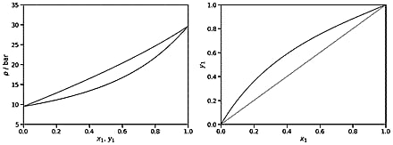
Similar to pure substance phase diagrams, there is a constructor for binary systems.
[27]: vle=feos.PhaseDiagram.binary_vle(eos,350*si.KELVIN,npoints=50)[28]: fig,ax=plt.subplots(1,2,figsize=(18,6))# fig.title("T = 350 K, Propane (1), Butane (2)")sns.lineplot(x=vle.liquid.molefracs[:,0],y=vle.liquid.pressure/si.BAR,ax=ax[0])sns.lineplot(x=vle.vapor.molefracs[:,0],y=vle.vapor.pressure/si.BAR,ax=ax[0])ax[0].set_xlabel(r"$x_1$, $y_1$")ax[0].set_ylabel(r"$p$ / bar")ax[0].set_xlim(0,1)ax[0].set_ylim(5,35)# ax[0].legend(frameon=False);sns.lineplot(x=vle.liquid.molefracs[:,0],y=vle.vapor.molefracs[:,0],ax=ax[1])sns.lineplot(x=np.linspace(0,1,10),y=np.linspace(0,1,10),color="black",alpha=0.3,ax=ax[1])ax[1].set_xlabel(r"$x_1$")ax[1].set_ylabel(r"$y_1$")ax[1].set_xlim(0,1)ax[1].set_ylim(0,1);
Comparison to Rust implementation
Implementing an equation of state in Python is nice for quick prototyping and development but when it comes to performance, implementing the equation of state in Rust is the way to go. For each non-cached call to the Helmholtz energy, we have to transition between Rust and Python with our Python implementation which generates quite some overhead.
Here are some comparisons between the Rust and our Python implemenation:
[29]: # rusteos_rust=feos.EquationOfState.peng_robinson(feos.Parameters.from_json(["propane"],"../../../examples/data/peng-robinson.json"))# pythontc=si.array(369.96*si.KELVIN)pc=si.array(4250000.0*si.PASCAL)omega=np.array([0.153])molar_weight=si.array(44.0962*si.GRAM/si.MOL)eos_python=feos.EquationOfState.python_residual(PyPengRobinson(tc,pc,omega,molar_weight))[30]: # let's first test if both actually yield the same results ;)assertabs(feos.State.critical_point(eos_python).pressure()/si.BAR-feos.State.critical_point(eos_rust).pressure()/si.BAR)<1e-12assertabs(feos.State.critical_point(eos_python).temperature/si.KELVIN-feos.State.critical_point(eos_rust).temperature/si.KELVIN)<1e-12[31]: importtimeittime_python=timeit.timeit(lambda:feos.State.critical_point(eos_python),number=2_500)time_rust=timeit.timeit(lambda:feos.State.critical_point(eos_rust),number=2_500)[32]: rel_dev=(time_rust-time_python)/time_rustprint(f"Critical point for pure substance")print(f"Python implementation is {'slower'ifrel_dev<0else'faster'} by a factor of {abs(time_python/time_rust):.0f}.")Critical point for pure substance Python implementation is slower by a factor of 23. [33]: time_python=timeit.timeit(lambda:feos.PhaseDiagram.pure(eos_python,300*si.KELVIN,100),number=100)time_rust=timeit.timeit(lambda:feos.PhaseDiagram.pure(eos_rust,300*si.KELVIN,100),number=100)[34]: rel_dev=(time_rust-time_python)/time_rustprint(f"Phase diagram for pure substance")print(f"Python implementation is {'slower'ifrel_dev<0else'faster'} by a factor of {abs(time_python/time_rust):.0f}.")Phase diagram for pure substance Python implementation is slower by a factor of 85.