Entropy scaling of pure substances
Goal
Learn how to compute dynamic properties (viscosity in this example)
Compare substance specific parameters against homo-segmented group contribution
Compare viscosity to NIST data (generated in NIST’s
)
Import needed packages
[1]: importfeosimportmatplotlib.pyplotaspltimportseabornassnsimportnumpyasnpimportpandasaspdimportsi_unitsassisns.set_context("talk")sns.set_palette("Dark2")sns.set_style("ticks")PC-SAFT (individual component parameters)
First, we read parameters adjusted to hexane saturation pressure and liquid densities (for the regular SAFT parameters) and to viscosity (for correlation).
[2]: parameters=feos.Parameters.from_json(["hexane"],"../../../parameters/pcsaft/loetgeringlin2018.json")parameters[2]: component
molarweight
m
sigma
epsilon_k
viscosity
hexane
86.177
3.0576
3.7983
236.77
[-1.2035,-2.5958,-0.4816,-0.0865]
PC-SAFT homo-GC
For transparency, we build parameters by hand. You can read a detailed explanation about PC-SAFT parameters in the “working with parameters” tutorial.
[3]: hexane=feos.ChemicalRecord(identifier=feos.Identifier(cas="110-54-3",name="hexane",iupac_name="hexane",smiles="CCCCCC",inchi="InChI=1/C6H14/c1-3-5-6-4-2/h3-6H2,1-2H3",formula="C6H14"),segments=['CH3','CH2','CH2','CH2','CH2','CH3'])ch3=feos.SegmentRecord('CH3',molarweight=15.0345,m=0.61198,sigma=3.7202,epsilon_k=229.90,viscosity=[-8.6878e-3,-1.7951e-1,-12.2359e-2,-0.01245])ch2=feos.SegmentRecord('CH2',molarweight=14.02658,m=0.45606,sigma=3.8900,epsilon_k=239.01,viscosity=[-0.9194e-3,-1.3316e-1,-4.2657e-2,-0.01245])segment_records={r.identifier:rforrin[ch3,ch2]}deffrom_segments(chemical_record,segment_records):m=0s3=0eps=0mw=0viscosity=np.zeros(4)forsinchemical_record.segments:segment=segment_records[s]mw+=segment.molarweightm+=segment.model_record["m"]s3+=segment.model_record["m"]*segment.model_record["sigma"]**3eps+=segment.model_record["m"]*segment.model_record["epsilon_k"]v=segment.model_record["viscosity"]viscosity+=np.array([v[0]*segment.model_record["m"]*segment.model_record["sigma"]**3,v[1]*segment.model_record["m"]*segment.model_record["sigma"]**3,v[2],v[3]])viscosity[1]/=s3**0.45# We have to shift the "A" parameter because the implemented reference# is eta_CE according to eq. 3 of Loetgerin-Lin (2018)# A = A(GC) + log(sqrt(1/m)) = -log(m)/2viscosity[0]+=np.log(np.sqrt(1/m))returnfeos.PureRecord(chemical_record.identifier,mw,m=m,sigma=np.cbrt(s3/m),epsilon_k=eps/m,viscosity=list(viscosity))Build equations of state
We instantiate an equation of state for each parameter set. saft uses substance specific parameters while saft_gc uses homo GC parameters both for SAFT as well as correlation parameters.
[4]: parameters_gc=feos.Parameters.new_pure(from_segments(hexane,segment_records))saft_gc=feos.EquationOfState.pcsaft(parameters_gc)saft=feos.EquationOfState.pcsaft(parameters)m_gc=parameters_gc.pure_records[0].model_record["m"]m=parameters.pure_records[0].model_record["m"]Compare parameters
[5]: print("Substance specific: ",parameters.pure_records[0].model_record["viscosity"])print("Segments : ",parameters_gc.pure_records[0].model_record["viscosity"])Substance specific: [-1.2035, -2.5958, -0.4816, -0.0865] Segments : [-1.2034921145837285, -2.536713016411593, -0.415346, -0.0747] Compare methods to NIST data (T = 450 K)
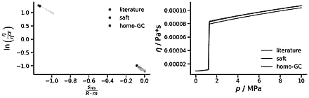
We will compute the residual entropy, viscosity and logarithmic reduced viscosity and compare to literature data (for which the entropy is computed with parameters fitted to the component, not GC).
[6]: literature=pd.read_csv("../../../examples/data/hexane_nist.csv",delimiter="\t")literature.head()[6]: Temperature (K)Pressure (MPa)Density (mol/m3)Volume (m3/mol)Internal Energy (kJ/mol)Enthalpy (kJ/mol)Entropy (J/mol*K)Cv (J/mol*K)Cp (J/mol*K)Sound Spd. (m/s)Joule-Thomson (K/MPa)Viscosity (Pa*s)Therm. Cond. (W/m*K)Phase0450.00.012.67740.37350045.22948.964154.33193.37201.76212.4711.2040.0000090.029374vapor1450.00.1129.98400.03335145.06548.734134.03193.94203.09209.0411.5100.0000090.029276vapor2450.00.2158.32900.01714444.89648.496128.27194.53204.55205.4811.8420.0000090.029196vapor3450.00.3187.82600.01138644.72048.249124.64195.15206.15201.7612.2070.0000090.029136vapor4450.00.41118.61000.00843144.53647.992121.90195.80207.93197.8712.6080.0000100.029098vaporWe loop through experimental data, read temperature, pressure and the phase (liquid or vapor) and generate State objects for the experimental conditions. Then, we compute the residual molar entropy and the logarithmic reduced viscosity.
[7]: results=[]fori,rowinliterature.iterrows():t=row['Temperature (K)']*si.KELVINp=row['Pressure (MPa)']*si.MEGA*si.PASCALviscosity_lit=row['Viscosity (Pa*s)']*si.PASCAL*si.SECOND# literaturestate=feos.State(saft,temperature=t,pressure=p,density_initialization=row.Phase)s=state.molar_entropy(feos.Contributions.Residual)results.append({"pressure":p/si.MEGA/si.PASCAL,"s*_res/m":s/si.RGAS/m,"viscosity":viscosity_lit/(si.PASCAL*si.SECOND),"ln_viscosity_reduced":np.log(viscosity_lit/state.viscosity_reference()),"source":"literature","rel.dev.":0.0})# individual parametersviscosity=state.viscosity()ln_viscosity_reduced=state.ln_viscosity_reduced()results.append({"pressure":p/si.MEGA/si.PASCAL,"s*_res/m":s/si.RGAS/m,"viscosity":viscosity/(si.PASCAL*si.SECOND),"ln_viscosity_reduced":ln_viscosity_reduced,"source":"saft","rel.dev.":(viscosity-viscosity_lit)/viscosity_lit*100})# homo GCstate=feos.State(saft_gc,temperature=t,pressure=p)s=state.molar_entropy(feos.Contributions.Residual)viscosity=state.viscosity()ln_viscosity_reduced=state.ln_viscosity_reduced()results.append({"pressure":p/si.MEGA/si.PASCAL,"s*_res/m":s/si.RGAS/m_gc,"viscosity":viscosity/(si.PASCAL*si.SECOND),"ln_viscosity_reduced":ln_viscosity_reduced,"source":"homo-GC","rel.dev.":(viscosity-viscosity_lit)/viscosity_lit*100})# gather everything in a data framedata=pd.DataFrame(results)data.head()[7]: pressures*_res/mviscosityln_viscosity_reducedsourcerel.dev.00.01-0.0005260.000009-1.170829literature0.00000010.01-0.0005260.000009-1.202136saft-3.08213020.01-0.0005310.000009-1.202146homo-GC-4.15434230.11-0.0058620.000009-1.172124literature0.00000040.11-0.0058620.000009-1.188299saft-1.604523[8]: fig,ax=plt.subplots(1,2,figsize=(15,4),gridspec_kw={'wspace':0.35})sns.scatterplot(data=data,x='s*_res/m',y='ln_viscosity_reduced',hue='source',ax=ax[0])ax[0].set_xlabel(r"$\frac{s_{res}}{R \cdot m}$",fontsize=22)ax[0].set_ylabel(r"$\ln\left(\frac{\eta}{\eta^{CE}}\right)$",fontsize=22)ax[0].legend(frameon=False)sns.lineplot(data=data,x='pressure',y='viscosity',hue='source',ax=ax[1])ax[1].set_xlabel(r"$p$ / MPa",fontsize=22)ax[1].set_ylabel(r"$\eta$ / Pa*s",fontsize=22)ax[1].legend(frameon=False)sns.despine()
[9]: # check mean absolute relative deviation in percentmard=data.groupby('source')['rel.dev.'].apply(lambdax:np.mean(np.abs(x)))print('Viscosity hexane compared to NIST data at T = 450 K')print(f'MARD (individual): {mard.saft:.2f} %')print(f'MARD (homo-GC) : {mard["homo-GC"]:.2f} %')Viscosity hexane compared to NIST data at T = 450 K MARD (individual): 0.81 % MARD (homo-GC) : 3.70 %