GitHub - xarray-contrib/xarray-spatial: Spatial analysis algorithms for xarray implemented in numba
Important
xarray-spatial uses AI assistance more aggressively than other open-source projects. Before opening a PR, read the
AI-Assisted Contribution Policy
and run your changes through the project's approved AI review workflow (see the command suite in the
repo). PRs that ignore the workflow are likely to be rejected.
Feature freeze in effect. The project is working toward its first major release (1.0.0). Until 1.0.0 ships, only bug fixes, test coverage, performance work, and documentation PRs will be considered. New feature proposals will be triaged but not implemented until after the release.
Contributors Wanted!. xarray-spatial is currently looking for contributors to help run pre-defined AI-assisted workflows as we approach v1.0.0. If you are interested, please add an issue and flag @brendancol and we can chat.
Latest Release
Downloads
License
People
Build Status


Coverage
———

📍 Fast, Accurate Python library for Raster Operations
⚡ Extensible with
⏩ Scalable with
🖥️ GPU-accelerated with
and
🎊 Free of GDAL / GEOS Dependencies
🌍 General-Purpose Spatial Processing, Geared Towards GIS Professionals
———
Xarray-Spatial is a Python library for raster analysis built on xarray. It has 150+ functions for surface analysis, hydrology (D8, D-infinity, MFD), fire behavior, flood modeling, multispectral indices, proximity, classification, pathfinding, and interpolation. Functions dispatch automatically across four backends (NumPy, Dask, CuPy, Dask+CuPy). A built-in GeoTIFF/COG reader and writer handles raster I/O without GDAL.
Installation
# via pip pip install xarray-spatial # with plotting helpers (matplotlib) pip install xarray-spatial[plot] # with vector rasterization (shapely): rasterize, polygonize pip install xarray-spatial[vector] # via conda conda install -c conda-forge xarray-spatialDownloading our starter examples and data
Once you have xarray-spatial installed in your environment, you can use one of the following in your terminal (with the environment active) to download our examples and/or sample data into your local directory.
xrspatial examples : Download the examples notebooks and the data used.
xrspatial copy-examples : Download the examples notebooks but not the data. Note: you won't be able to run many of the examples.
xrspatial fetch-data : Download just the data and not the notebooks.
In all the above, the command will download and store the files into your current directory inside a folder named 'xrspatial-examples'.
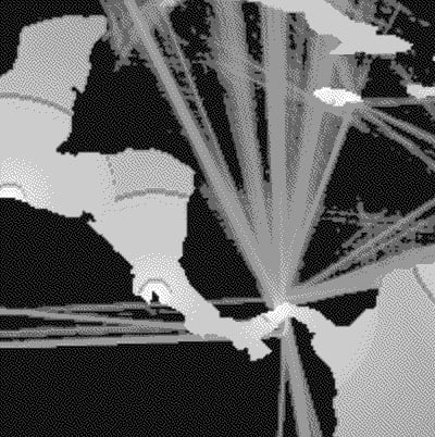


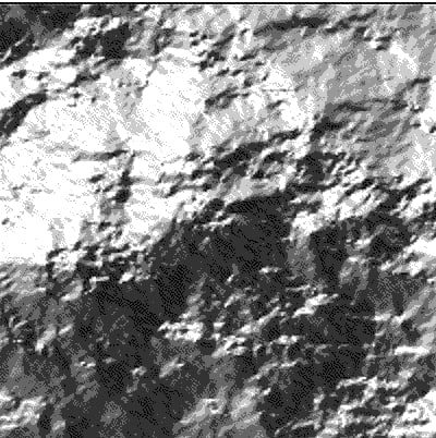
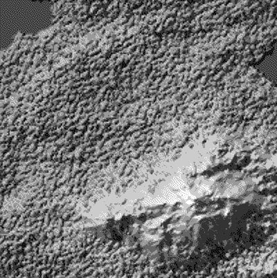
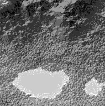

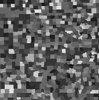
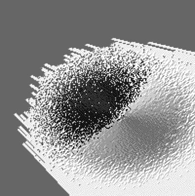
xarray-spatial grew out of the
, which provides fast rasterization of vector data (points, lines, polygons, meshes, and rasters) for use with xarray-spatial.
xarray-spatial does not depend on GDAL or GEOS. Raster I/O, reprojection, compression codecs, and coordinate handling are all pure Python and Numba -- no C/C++ bindings anywhere in the stack.
and
cover every module.
Raster-huh?
Rasters are regularly gridded datasets like GeoTIFFs, JPGs, and PNGs.
In the GIS world, rasters are used for representing continuous phenomena (e.g. elevation, rainfall, distance), either directly as numerical values, or as RGB images created for humans to view. Rasters typically have two spatial dimensions, but may have any number of other dimensions (time, type of measurement, etc.)
Supported Spatial Functions with Supported Inputs
Each cell shows the feature tier for that function on that backend (see
). A blank cell means no implementation on that backend; a path that was previously documented as a CPU fallback is reported here as advanced (it works as a documented execution mode, but is not native-parity tested).
✅ stable · 🔼 advanced · 🧪 experimental · 🔧 internal · 🚫 unsupported
·
·
·
·
·
·
·
·
·
·
·
·
·
·
·
·
·
·
·
·
———
GeoTIFF / COG I/O
Native GeoTIFF and Cloud Optimized GeoTIFF reader/writer. No GDAL required.
VRT is supported as a conservative advanced feature for simple GeoTIFF mosaics, not as a full GDAL VRT replacement. See the
for the supported subset and what is out of scope.
NameDescriptionNumPyDaskCuPy GPUDask+CuPy GPUCloud
Read GeoTIFF / COG / VRT✅✅🧪🧪🔼
Write DataArray as GeoTIFF / COG / VRT✅✅🧪🧪🔼open_geotiff and to_geotiff select the backend from their parameters (gpu=, chunks=, .vrt path); GPU read/write is reached with gpu=True, not a separate function:
fromxrspatial.geotiffimportopen_geotiff, to_geotiffopen_geotiff('dem.tif') # NumPyopen_geotiff('dem.tif', chunks=512) # Daskopen_geotiff('dem.tif', gpu=True) # CuPy (nvCOMP + GDS)open_geotiff('dem.tif', gpu=True, chunks=512) # Dask + CuPyopen_geotiff('https://example.com/cog.tif') # HTTP COGopen_geotiff('s3://bucket/dem.tif') # Cloud (S3/GCS/Azure)open_geotiff('mosaic.vrt') # VRT mosaic (auto-detected)to_geotiff(cupy_array, 'out.tif') # auto-detects GPUto_geotiff(data, 'out.tif', gpu=True) # force GPU compressto_geotiff(data, 'out.tif', compression='zstd') # ZSTD for smaller filesto_geotiff(data, 'cog.tif', cog=True) # COG with auto overviewsto_geotiff(data, 'cog.tif', cog=True, # COG with explicit levelsoverview_levels=[2, 4, 8], overview_resampling='nearest') to_geotiff(data, 'mosaic.vrt') # write a tiled VRT mosaicopen_geotiff('dem.tif', dtype='float32') # half memoryopen_geotiff('dem.tif', dtype='float32', chunks=512) # Dask + half memoryto_geotiff(data, 'out.tif', compression_level=1) # fast scratch writeto_geotiff(data, 'out.tif', compression_level=22) # max compressionto_geotiff(dask_da, 'out.tif') # stream Dask to single TIFFto_geotiff(dask_da, 'mosaic.vrt') # stream Dask to VRT# Accessor methodsda.xrs.to_geotiff('out.tif', compression='lzw') # write from DataArrayds.xrs.open_geotiff('large_dem.tif') # read windowed to Dataset extent# xarray backend engineimportxarrayasxrxr.open_dataset('dem.tif', engine='xrspatial') # open as a Datasetxr.open_mfdataset('*.tif', engine='xrspatial', # share one var namebackend_kwargs={'default_name': 'band_data'})Compression codecs: Deflate, LZW (Numba JIT), ZSTD, PackBits, JPEG (Pillow, internal-only: requires allow_internal_only_jpeg=True and is not readable by GDAL), JPEG 2000 (glymur, experimental: requires allow_experimental_codecs=True), uncompressed
GPU codecs: Deflate and ZSTD via nvCOMP batch API; JPEG 2000 via nvJPEG2000; LZW via Numba CUDA kernels
Features:
Tiled, stripped, BigTIFF, multi-band (RGB/RGBA), sub-byte (1/2/4/12-bit)
Predictors: horizontal differencing (pred=2), floating-point (pred=3)
GeoKeys: EPSG, WKT/PROJ (via pyproj), citations, units, ellipsoid, vertical CRS
Metadata: nodata masking, palette colormaps, DPI/resolution, GDALMetadata XML, arbitrary tag preservation
Cloud storage: S3 (s3://), GCS (gs://), Azure (az://) via fsspec
GPUDirect Storage: SSD→GPU direct DMA via KvikIO (optional)
Thread-safe mmap reads, atomic writes, HTTP connection reuse (urllib3)
Overview generation (CPU and GPU): mean, nearest, min, max, median, mode, cubic
Planar config, big-endian byte swap, PixelIsArea/PixelIsPoint
Consistency: 100% pixel-exact match vs rioxarray on all tested files (Landsat 8, Copernicus DEM, USGS 1-arc-second, USGS 1-meter).
———
Reproject / Merge / Resample
NameDescriptionSourceNumPy xr.DataArrayDask xr.DataArrayCuPy GPU xr.DataArrayDask GPU xr.DataArray
Changes raster resolution (cell size) without reprojection. Nearest, bilinear, cubic, average, mode, min, max, median methodsStandard (interpolation / block aggregation)✅🔼🔼🔼
Reprojects a raster to a new CRS with Numba JIT / CUDA coordinate transforms and resampling. Supports vertical datums (EGM96, EGM2008) and horizontal datum shifts (NAD27, OSGB36, etc.)Standard (inverse mapping)✅🔼🔼🔼
Merges multiple rasters into a single mosaic with configurable overlap strategy. Same-CRS tiles skip reprojection and are placed by direct coordinate alignmentStandard (mosaic)🔼🔼🔼🔼Built-in Numba JIT and CUDA projection kernels bypass pyproj for per-pixel coordinate transforms. pyproj is used only for CRS metadata parsing (~1ms, once per call) and output grid boundary estimation (~500 control points, once per call). Any CRS pair without a built-in kernel falls back to pyproj automatically.
ProjectionEPSG examplesCPU NumbaCUDA GPUWeb Mercator3857✅️✅️UTM / Transverse Mercator326xx, 327xx, State Plane✅️✅️Ellipsoidal Mercator3395✅️✅️Lambert Conformal Conic2154, 2229, State Plane✅️✅️Albers Equal Area5070✅️✅️Cylindrical Equal Area6933✅️✅️SinusoidalMODIS grids✅️✅️Lambert Azimuthal Equal Area3035, 6931, 6932✅️✅️Polar Stereographic3031, 3413, 3996✅️✅️Oblique Stereographiccustom WGS84✅️pyproj fallbackOblique Mercator (Hotine)3375 (RSO)implemented, disabledpyproj fallbackVertical datum support:geoid_height, ellipsoidal_to_orthometric, orthometric_to_ellipsoidal convert between ellipsoidal (GPS) and orthometric (map/MSL) heights using EGM96 (vendored, 2.6MB) or EGM2008 (77MB, downloaded on first use). Reproject can apply vertical shifts during reprojection via the vertical_crs parameter.
Datum shift support: Reprojection from non-WGS84 datums (NAD27, OSGB36, DHDN, MGI, ED50, BD72, CH1903, D73, AGD66, Tokyo) applies grid-based shifts from PROJ CDN (sub-metre accuracy) with 7-parameter Helmert fallback (1-5m accuracy). 14 grids are registered covering North America, UK, Germany, Austria, Spain, Netherlands, Belgium, Switzerland, Portugal, and Australia.
ITRF frame support:itrf_transform converts between ITRF2000, ITRF2008, ITRF2014, and ITRF2020 using 14-parameter time-dependent Helmert transforms from PROJ data files. Shifts are mm-level.
———
Utilities
NameDescriptionSourceNumPy xr.DataArrayDask xr.DataArrayCuPy GPU xr.DataArrayDask GPU xr.DataArray
Downsamples a raster to target pixel dimensions for visualizationCustom✅🔼🔼🔼
Min-max normalization to a target range (default [0, 1])Standard✅🔼🔼🔼
Z-score normalization (subtract mean, divide by std)Standard✅🔼🔼🔼
Rechunk dask arrays using whole-chunk multiples (no shuffle)Custom🔼🔼🔼🔼
Fuse sequential map_overlap calls into a single passCustom🔼🔼🔼🔼
Run multi-output kernel in a single overlap passCustom🔼🔼🔼🔼
Check a raster against the xarray-spatial input contract (.xrs.validate())Custom✅🔼🔼🔼
———
Templates
NameDescriptionSourceNumPy xr.DataArrayDask xr.DataArrayCuPy GPU xr.DataArrayDask GPU xr.DataArray
Empty study-area grid for a named region (CONUS, NYC, ...), a world city (London, Tokyo, ... in its UTM zone), a country code, or a whole-world projection (web_mercator, wgs84/latlon, equal_earth); preserve='area'/'shape' picks an EPSG projection by property; list_templates() lists every accepted nameCustom✅🔼🔼🔼
———
Surface
NameDescriptionSourceNumPy xr.DataArrayDask xr.DataArrayCuPy GPU xr.DataArrayDask GPU xr.DataArray
Computes downslope direction of each cell in degreesHorn 1981✅🔼🔼🔼
North-south component of aspect: cos(aspect) for linear modelsStage 1976✅🔼🔼🔼
East-west component of aspect: sin(aspect) for linear modelsStage 1976✅🔼🔼🔼
Measures rate of slope change (concavity/convexity) at each cellZevenbergen & Thorne 1987✅🔼🔼🔼
Simulates terrain illumination from a given sun angle and azimuthGDAL gdaldem✅🔼🔼🔼
Computes local relief as max minus min elevation in a 3×3 windowGDAL gdaldem✅🔼🔼🔼
Measures the fraction of visible sky hemisphere at each cellZakek et al. 2011✅🔼🔼🔼
Computes terrain gradient steepness at each cell in degreesHorn 1981✅🔼🔼🔼
Generates synthetic terrain from fBm or ridged fractal noise with optional domain warping, Worley blending, and hydraulic erosionCustom (fBm)🔼🔼🔼🔼
Computes Topographic Position Index (center minus mean of neighbors)Weiss 2001✅🔼🔼🔼
Computes Terrain Ruggedness Index (local elevation variation)Riley et al. 1999✅🔼🔼🔼
Classifies terrain into 10 landform types using the Weiss (2001) TPI schemeWeiss 2001✅🔼🔼🔼
Determines visible cells from a given observer point on terrainGRASS GIS r.viewshed🔼🔼🔼🔼
Counts how many observers can see each cellCustom🔼🔼🔼🔼
Fraction of observers with line-of-sight to each cellCustom🔼🔼🔼🔼
Elevation profile and visibility along a point-to-point transectCustom🔼🔼🔼🔼
Finds the minimum observer height needed to see each cellCustom🧪
Generates smooth continuous random noise for procedural texturesPerlin 1985✅🔼🔼🔼
Generates cellular (Voronoi) noise returning distance to the nearest feature pointWorley 1996✅🔼🔼🔼
Simulates particle-based water erosion to carve valleys and deposit sedimentCustom🔼🔼🔼🔼
Adds randomized bump features to simulate natural terrain variationCustom🔼🔼🔼🔼
———
Hydrology
NameDescriptionSourceNumPy xr.DataArrayDask xr.DataArrayCuPy GPU xr.DataArrayDask GPU xr.DataArray
Direction of steepest descent out of each cell (D8 · Dinf · MFD via routing=)O'Callaghan & Mark 1984; Tarboton 1997; Qin et al. 2007✅🔼🔼🔼
Upstream cells or area draining through each cell (D8 · Dinf · MFD via routing=)Jenson & Domingue 1988; Tarboton 1997; Qin et al. 2007✅🔼🔼🔼
Flow path length to the outlet or from the divide (D8 · Dinf · MFD via routing=)Tarboton 1997; Qin et al. 2007🔼🔼🔼🔼
Traces downstream flow paths from start points (D8 · Dinf · MFD via routing=)Tarboton 1997; Qin et al. 2007🔼🔼🔼🔼
Labels each cell with the pour point it drains to (D8 · Dinf · MFD via routing=)Tarboton 1997; Qin et al. 2007✅🔼🔼🔼
Assigns unique IDs to stream segments above a threshold (D8 · Dinf · MFD via routing=)Tarboton 1997; Freeman 1991✅🔼🔼🔼
Strahler or Shreve stream ordering of the network (D8 · Dinf · MFD via routing=)Strahler 1957, Shreve 1966✅🔼🔼🔼
Height Above Nearest Drainage (D8 · Dinf · MFD via routing=)Nobre et al. 2011✅🔼🔼🔼
Fills depressions in a DEM using Planchon-Darboux iterative flooding (D8)Planchon & Darboux 2002✅🔼🔼🔼
Identifies and labels depression cells (D8)Standard (D8 tracing)✅🔼🔼🔼
Labels each cell with the outlet of the basin it drains to (D8)Standard (D8 tracing)✅🔼🔼🔼
Snaps pour points to the highest-accumulation cell within a search radius (D8)Custom✅🔼🔼🔼
Topographic Wetness Index: ln(specific catchment area / tan(slope)) (D8)Beven & Kirkby 1979✅🔼🔼🔼
———
Flood
NameDescriptionSourceNumPy xr.DataArrayDask xr.DataArrayCuPy GPU xr.DataArrayDask GPU xr.DataArray
Computes water depth above terrain from a HAND raster and water levelStandard (HAND-based)✅🔼🔼🔼
Produces a binary flood/no-flood mask from a HAND raster and water levelStandard (HAND-based)✅🔼🔼🔼
Estimates runoff depth from rainfall using the SCS/NRCS curve number methodSCS/NRCS✅🔼🔼🔼
Estimates overland flow travel time via simplified Manning's equationManning 1891✅🔼🔼🔼
Derives Manning's roughness coefficients from NLCD land cover or NDVISCS/NRCS✅🔼🔼🔼
Derives SCS curve numbers from land cover and hydrologic soil groupSCS/NRCS✅🔼🔼🔼
Manning-based steady-state flow depth incorporating vegetation roughnessManning 1891✅🔼🔼🔼
———
Multispectral
NameDescriptionSourceNumPy xr.DataArrayDask xr.DataArrayCuPy GPU xr.DataArrayDask GPU xr.DataArray
Atmospherically Resistant Vegetation Index (ARVI)
Vegetation index resistant to atmospheric effects using blue band correctionKaufman & Tanre 1992✅🔼🔼🔼
Spectral distance to charcoal reflectance point for burn scar detectionChuvieco et al. 2002✅🔼🔼🔼
Enhanced Built-Up and Bareness Index (EBBI)
Highlights built-up areas and barren land from thermal and SWIR bandsAs-syakur et al. 2012✅🔼🔼🔼
Enhanced Vegetation Index (EVI)
Enhanced vegetation index reducing soil and atmospheric noiseHuete et al. 2002✅🔼🔼🔼
Estimates leaf chlorophyll content from green and NIR reflectanceGitelson et al. 2003✅🔼🔼🔼
Modified Soil Adjusted Vegetation Index (MSAVI2)
Self-adjusting soil line vegetation index, no L parameter neededQi et al. 1994✅🔼🔼🔼
Measures burn severity using NIR and SWIR band differenceUSGS Landsat✅🔼🔼🔼
Normalized Burn Ratio 2 (NBR2)
Refines burn severity mapping using two SWIR bandsUSGS Landsat✅🔼🔼🔼
Normalized Difference Built-up Index (NDBI)
Picks out built-up and urban areas from SWIR and NIR bandsZha et al. 2003✅🔼🔼🔼
Normalized Difference Moisture Index (NDMI)
Detects vegetation moisture stress from NIR and SWIR reflectanceUSGS Landsat✅🔼🔼🔼
Normalized Difference Snow Index (NDSI)
Separates snow and ice from clouds using green and SWIR bandsHall et al. 1995✅🔼🔼🔼
Normalized Difference Water Index (NDWI)
Maps open water bodies using green and NIR band differenceMcFeeters 1996✅🔼🔼🔼
Modified Normalized Difference Water Index (MNDWI)
Detects water in urban areas using green and SWIR bandsXu 2006✅🔼🔼🔼
Normalized Difference Vegetation Index (NDVI)
Quantifies vegetation density from red and NIR band differenceRouse et al. 1973✅🔼🔼🔼
Optimized Soil Adjusted Vegetation Index (OSAVI)
SAVI with fixed L=0.16, tuned for sparse vegetationRondeaux et al. 1996✅🔼🔼🔼
Soil Adjusted Vegetation Index (SAVI)
Vegetation index with soil brightness correction factorHuete 1988✅🔼🔼🔼
Structure Insensitive Pigment Index (SIPI)
Estimates carotenoid-to-chlorophyll ratio for plant stress detectionPenuelas et al. 1995✅🔼🔼🔼
Composites red, green, and blue bands into a natural color imageStandard✅🔼🔼🔼For a broader catalog of spectral indices and sensor-specific band combinations, see
and its companion xarray library
.
———
Classification
NameDescriptionSourceNumPy xr.DataArrayDask xr.DataArrayCuPy GPU xr.DataArrayDask GPU xr.DataArray
Binarizes values by membership in a target set (1 if match, 0 otherwise)Standard✅🔼🔼🔼
Classifies values into bins based on box plot quartile boundariesPySAL mapclassify✅🔼🔼🔼
Divides the value range into equal-width binsPySAL mapclassify✅🔼🔼🔼
Classifies heavy-tailed distributions using recursive mean splittingPySAL mapclassify✅🔼🔼🔼
Finds natural groupings by maximizing differences between sorted valuesPySAL mapclassify✅🔼🔼🔼
Optimizes class boundaries to minimize within-class variance (Jenks)Jenks 1967, PySAL✅🔼🔼🔼
Assigns classes based on user-defined percentile breakpointsPySAL mapclassify✅🔼🔼🔼
Distributes values into classes with equal observation countsPySAL mapclassify✅🔼🔼🔼
Remaps pixel values to new classes using a user-defined lookupPySAL mapclassify✅🔼🔼🔼
Classifies values by standard deviation intervals from the meanPySAL mapclassify✅🔼🔼🔼
———
Focal
NameDescriptionSourceNumPy xr.DataArrayDask xr.DataArrayCuPy GPU xr.DataArrayDask GPU xr.DataArray
Applies a custom function over a sliding neighborhood windowStandard🔼🔼🔼🔼
Identifies statistically significant spatial clusters using Getis-Ord Gi*Getis & Ord 1992✅🔼🔼🔼
Classifies time-series hot/cold spot trends using Gi* and Mann-KendallGetis & Ord 1992, Mann 1945🔼🔼🔼🔼
Computes the mean value within a sliding neighborhood windowStandard✅🔼🔼🔼
Computes summary statistics over a sliding neighborhood windowStandard✅🔼🔼🔼
Feature-preserving smoothing via bilateral filteringTomasi & Manduchi 1998🔼🔼🔼🔼
Computes Haralick GLCM texture features over a sliding windowHaralick et al. 1973🔼🔼🔼🔼
Horizontal gradient via Sobel operator (detects vertical edges)Sobel & Feldman 1968🔼🔼🔼🔼
Vertical gradient via Sobel operator (detects horizontal edges)Sobel & Feldman 1968🔼🔼🔼🔼
Omnidirectional second-derivative edge detectorStandard🔼🔼🔼🔼
Horizontal gradient via Prewitt operator (detects vertical edges)Prewitt 1970🔼🔼🔼🔼
Vertical gradient via Prewitt operator (detects horizontal edges)Prewitt 1970🔼🔼🔼🔼
———
Proximity
NameDescriptionSourceNumPy xr.DataArrayDask xr.DataArrayCuPy GPU xr.DataArrayDask GPU xr.DataArray
Assigns each cell to the identity of the nearest source featureStandard (Dijkstra)✅🔼🔼🔼
Partitions a cost surface into territories of roughly equal cost-weighted areaCustom🔼🔼🔼🔼
Computes minimum accumulated cost to the nearest source through a friction surfaceStandard (Dijkstra)✅🔼🔼🔼
Identifies zones of low cumulative cost between two source locationsStandard (Dijkstra)🔼🔼🔼🔼
Computes the direction from each cell to the nearest source featureStandard✅🔼🔼🔼
Computes the distance from each cell to the nearest source featureStandard✅🔼🔼🔼
Computes distance along the 3D terrain surface to the nearest sourceStandard (Dijkstra)🔼🔼🔼🔼
Assigns each cell to the nearest source by terrain surface distanceStandard (Dijkstra)🔼🔼🔼🔼
Computes compass direction to the nearest source by terrain surface distanceStandard (Dijkstra)🔼🔼🔼🔼
———
Zonal
NameDescriptionSourceNumPy xr.DataArrayDask xr.DataArrayCuPy GPU xr.DataArrayDask GPU xr.DataArray
Applies a custom function to each zone in a classified rasterStandard🔼🔼🔼🔼
Clips a raster to an arbitrary polygon with maskingStandard🔼🔼🔼🔼
Extracts the bounding rectangle of a specific zoneStandard✅🔼🔼🔼
Identifies connected regions of non-zero cellsStandard (CCL)✅🔼🔼🔼
Removes nodata border rows and columns from a rasterStandard✅🔼🔼🔼
Computes summary statistics for a value raster within each zoneStandard✅🔼🔼🔼
Cross-tabulates agreement between two categorical rastersStandard🔼🔼🔼🔼
———
Interpolation
NameDescriptionSourceNumPy xr.DataArrayDask xr.DataArrayCuPy GPU xr.DataArrayDask GPU xr.DataArray
Inverse Distance Weighting from scattered points (arrays or a GeoDataFrame) to a raster gridStandard (IDW)✅🔼🔼🔼
Ordinary Kriging with automatic variogram fitting (spherical, exponential, gaussian); accepts arrays or a GeoDataFrameStandard (ordinary kriging)🔼🔼🔼🔼
Thin Plate Spline interpolation with optional smoothing; accepts arrays or a GeoDataFrameStandard (TPS)🔼🔼🔼🔼
———
Morphological
NameDescriptionSourceNumPy xr.DataArrayDask xr.DataArrayCuPy GPU xr.DataArrayDask GPU xr.DataArray
Morphological erosion (local minimum over structuring element)Standard (morphology)✅🔼🔼🔼
Morphological dilation (local maximum over structuring element)Standard (morphology)✅🔼🔼🔼
Erosion then dilation (removes small bright features)Standard (morphology)✅🔼🔼🔼
Dilation then erosion (fills small dark gaps)Standard (morphology)✅🔼🔼🔼
Dilation minus erosion (edge detection)Standard (morphology)✅🔼🔼🔼
Original minus opening (isolate bright features)Standard (morphology)✅🔼🔼🔼
Closing minus original (isolate dark features)Standard (morphology)✅🔼🔼🔼
Remove small connected clumps from classified rastersGDAL sieve🔼🔼🔼🔼
———
Fire
NameDescriptionSourceNumPy xr.DataArrayDask xr.DataArrayCuPy GPU xr.DataArrayDask GPU xr.DataArray
Differenced Normalized Burn Ratio (pre minus post NBR)USGS✅🔼🔼🔼
Relative dNBR normalized by pre-fire vegetation densityUSGS✅🔼🔼🔼
USGS 7-class burn severity from dNBR thresholdsUSGS✅🔼🔼🔼
Byram's fireline intensity from fuel load and spread rate (kW/m)Byram 1959✅🔼🔼🔼
Flame length derived from fireline intensity (m)Byram 1959✅🔼🔼🔼
Simplified Rothermel spread rate with Anderson 13 fuel models (m/min)Rothermel 1972, Anderson 1982✅🔼🔼🔼
Keetch-Byram Drought Index single time-step update (0-800 mm)Keetch & Byram 1968✅🔼🔼🔼
———
Raster / Vector Conversion
NameDescriptionSourceNumPy xr.DataArrayDask xr.DataArrayCuPy GPU xr.DataArrayDask GPU xr.DataArray
Converts contiguous regions of equal value into vector polygonsStandard (CCL)🔼🔼🔼🔼
Extracts elevation contour lines (isolines) from a raster surfaceStandard (marching squares)🔼🔼🔼🔼
Rasterizes vector geometries (polygons, lines, points) from a GeoDataFrameStandard (scanline, Bresenham)🔼🔼
———
Kernel Density Estimation
NameDescriptionSourceNumPy xr.DataArrayDask xr.DataArrayCuPy GPU xr.DataArrayDask GPU xr.DataArray
Point-to-raster kernel density estimation (Gaussian, Epanechnikov, quartic); accepts arrays or a GeoDataFrameSilverman 1986🔼🔼🔼🔼
Line-segment-to-raster density estimationStandard🔼
———
Multivariate
NameDescriptionSourceNumPy xr.DataArrayDask xr.DataArrayCuPy GPU xr.DataArrayDask GPU xr.DataArray
Measures statistical distance from a multi-band reference distribution, accounting for band correlationsMahalanobis 1936✅🔼🔼🔼
———
Multi-Criteria Decision Analysis (MCDA)
NameDescriptionSourceNumPy xr.DataArrayDask xr.DataArrayCuPy GPU xr.DataArrayDask GPU xr.DataArray
Converts criterion rasters to 0-1 suitability scale (linear, sigmoidal, gaussian, triangular, piecewise, categorical)Standard✅🔼🔼🔼
Derives criterion weights from pairwise comparisons using the Saaty eigenvector method with consistency ratioSaaty 1980✅🚫🚫🚫
Derives weights from a rank ordering (ROC, rank sum, reciprocal)Standard✅🚫🚫🚫
Weighted Linear Combination (fully compensatory weighted sum)Malczewski 2006✅🔼🧪🧪
Weighted Product Model (multiplicative, penalizes low scores)Standard✅🔼🧪🧪
Ordered Weighted Averaging with tunable risk attitudeYager 1988✅🔼🧪🧪
Combines criteria using fuzzy set operators (AND, OR, sum, product, gamma)Eastman 1999✅🔼🧪🧪
Combines binary criterion masks using AND/OR logicStandard✅🔼🧪🧪
Masks exclusion zones from a suitability surfaceStandard✅🔼🧪🧪
Assesses weight stability via one-at-a-time or Monte Carlo perturbationStandard✅🔼🧪🧪
———
Pathfinding
NameDescriptionSourceNumPy xr.DataArrayDask xr.DataArrayCuPy GPU xr.DataArrayDask GPU xr.DataArray
Finds the least-cost path between two cells on a cost surfaceHart et al. 1968✅🔼🔼🔼
Routes through N waypoints in sequence, with optional TSP reorderingCustom🔼🔼🔼🔼
———
Diffusion
NameDescriptionSourceNumPy xr.DataArrayDask xr.DataArrayCuPy GPU xr.DataArrayDask GPU xr.DataArray
Runs explicit forward-Euler diffusion on a 2D scalar fieldStandard (heat equation)✅🔼🔼🔼
———
Dasymetric
NameDescriptionSourceNumPy xr.DataArrayDask xr.DataArrayCuPy GPU xr.DataArrayDask GPU xr.DataArray
Redistributes zonal totals to pixels using an ancillary weight surfaceMennis 2003🔼🔼🔼🔼
Tobler's pycnophylactic interpolation preserving zone totals via Laplacian smoothingTobler 1979✅🚫🔼🚫
Checks that disaggregated pixel sums match the original zone totalsStandard✅🔼🔼🔼
———
Usage
Quick StartImporting xrspatial registers an .xrs accessor on DataArrays and Datasets, giving you tab-completable access to every spatial operation:
importxrspatialasxrsfromxrspatial.geotiffimportopen_geotiff, to_geotiff# Read a GeoTIFF (no GDAL required)elevation=open_geotiff('dem.tif') # Surface analysisslope=elevation.xrs.slope() hillshaded=elevation.xrs.hillshade(azimuth=315, angle_altitude=45) aspect=elevation.xrs.aspect() # Reproject and write as a Cloud Optimized GeoTIFFdem_wgs84=elevation.xrs.reproject(target_crs='EPSG:4326') to_geotiff(dem_wgs84, 'output.tif', cog=True) # Classificationclasses=elevation.xrs.equal_interval(k=5) breaks=elevation.xrs.natural_breaks(k=10) # Proximitydistance=elevation.xrs.proximity(target_values=[1]) # Multispectralvegetation=nir.xrs.ndvi(red) enhanced_vi=nir.xrs.evi(red, blue)Dataset SupportThe .xrs accessor works on Datasets too. Single-input functions apply the operation to each data variable. Multi-input functions (multispectral indices) accept string kwargs that map band aliases to variable names:
ds=xr.Dataset({'band_4': red, 'band_5': nir}) # Single-input: slope computed for each variableslope_ds=ds.xrs.slope() # Multi-input: map variable names to band parametersndvi_result=ds.xrs.ndvi(nir='band_5', red='band_4')Function Import StyleAll operations are also available as standalone functions:
importxrspatialasxrshillshaded=xrs.hillshade(elevation) slope_result=xrs.slope(elevation) vegetation=xrs.ndvi(nir, red)Check out the user guide
.
———
Dependencies
Core: numpy, numba, scipy, xarray, zstandard
Optional:
matplotlib — the .xrs.plot accessor helpers (pip install xarray-spatial[plot])
shapely — the vector-to-raster paths, rasterize and polygonize (pip install xarray-spatial[vector])
pyproj — WKT/PROJ CRS resolution
cupy — GPU acceleration
dask — out-of-core processing
libnvcomp — GPU batch decompression (deflate, ZSTD)
kvikio — GPUDirect Storage (SSD → GPU)
fsspec + s3fs/gcsfs/adlfs — cloud storage
libnvcomp and kvikio are not pulled in by the gpu extra. They are runtime dependencies of the GeoTIFF GPU read path and must be installed separately (typically via conda from the rapidsai/nvidia channels), since libnvcomp ships as a system library and kvikio requires a matching CUDA toolkit.
Notes on GDAL
xarray-spatial does not depend on GDAL. The built-in GeoTIFF/COG reader and writer (xrspatial.geotiff) handles raster I/O natively using only numpy, numba, and the standard library. This means:
Zero GDAL installation hassle.pip install xarray-spatial gets you everything needed to read and write GeoTIFFs, COGs, and VRT files.
Pure Python, fully extensible. All codec, header parsing, and metadata code is readable Python/Numba, not wrapped C/C++.
GPU-accelerated reads. With optional nvCOMP and nvJPEG2000, compressed tiles decompress directly on the GPU via CUDA -- something GDAL cannot do.
The native reader is pixel-exact against rasterio/GDAL across Landsat 8, Copernicus DEM, USGS 1-arc-second, and USGS 1-meter DEMs.
Citation
Cite this code:
xarray-contrib/xarray-spatial, https://github.com/xarray-contrib/xarray-spatial, ©2020-2026.