numpy.fft.fft — NumPy v2.6.dev0 Manual
fft.fft(a, n=None, axis=-1, norm=None, out=None)
Compute the one-dimensional discrete Fourier Transform.
This function computes the one-dimensional n-point discrete Fourier Transform (DFT) with the efficient Fast Fourier Transform (FFT) algorithm
.
Parameters:aarray_likeInput array, can be complex.
nint, optionalLength of the transformed axis of the output. If n is smaller than the length of the input, the input is cropped. If it is larger, the input is padded with zeros. If n is not given, the length of the input along the axis specified by axis is used.
axisint, optionalAxis over which to compute the FFT. If not given, the last axis is used.
norm{“backward”, “ortho”, “forward”}, optionalNormalization mode (see
). Default is “backward”. Indicates which direction of the forward/backward pair of transforms is scaled and with what normalization factor.
Added in version 1.20.0: The “backward”, “forward” values were added.
outcomplex ndarray, optionalIf provided, the result will be placed in this array. It should be of the appropriate shape and dtype.
Added in version 2.0.0.
Returns:outcomplex ndarrayThe truncated or zero-padded input, transformed along the axis indicated by axis, or the last one if axis is not specified.
Raises:IndexErrorIf axis is not a valid axis of a.
See also
for definition of the DFT and conventions used.
The inverse of
.
The two-dimensional FFT.
The n-dimensional FFT.
The n-dimensional FFT of real input.
Frequency bins for given FFT parameters.
Notes
FFT (Fast Fourier Transform) refers to a way the discrete Fourier Transform (DFT) can be calculated efficiently, by using symmetries in the calculated terms. The symmetry is highest when n is a power of 2, and the transform is therefore most efficient for these sizes.
The DFT is defined, with the conventions used in this implementation, in the documentation for the
module.
References
[
]
Cooley, James W., and John W. Tukey, 1965, “An algorithm for the machine calculation of complex Fourier series,” Math. Comput. 19: 297-301.
Examples
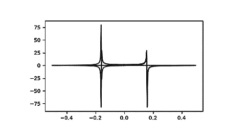
>>> importnumpyasnp>>> np.fft.fft(np.exp(2j*np.pi*np.arange(8)/8))array([-2.33486982e-16+1.14423775e-17j, 8.00000000e+00-1.25557246e-15j, 2.33486982e-16+2.33486982e-16j, 0.00000000e+00+1.22464680e-16j, -1.14423775e-17+2.33486982e-16j, 0.00000000e+00+5.20784380e-16j, 1.14423775e-17+1.14423775e-17j, 0.00000000e+00+1.22464680e-16j])In this example, real input has an FFT which is Hermitian, i.e., symmetric in the real part and anti-symmetric in the imaginary part, as described in the
documentation:
>>> importmatplotlib.pyplotasplt>>> t=np.arange(256)>>> sp=np.fft.fft(np.sin(t))>>> freq=np.fft.fftfreq(t.shape[-1])>>> _=plt.plot(freq,sp.real,freq,sp.imag)>>> plt.show()